Information in spiking neurons on latent variables

Originally published on Memming’s Substack

---

How many neurons do we need to simulatenously record from a brain region to reliably estimate a 5 dimensional continuous latent trajectory? Which neurons are more informative about the latent variables, and which ones are useless? These are important questions in experimental design and assessing quality of datasets.

Point process observations, such as neural spike trains, are completely characterized by their conditional intensity function:

\[\lambda(t; \mathcal{H}_t) = \lim_{\Delta t \to 0} \mathrm{Pr}\left[ \mathbf{N}(t, t+\Delta t)\right] / \Delta t\]

where N is the stochastic process that counts the number of spikes in a small time bin (Daley & Vere-Jones 1998).

In the state-space formulation, the conditional intensity function depends on the history via the Markovian latent neural state. In the field of neuroscience, the standard form of probabilistic observation model for spiking neuron (in a finite time bin) has the following form:

\[y_i(t) \sim \text{Poisson}\left( \exp(\mathbf{C_i} \mathbf{x}(t) + b_i) \right)\]

where y is the spike count of neuron i, x(t) is the latent process, C is the loading matrix, b is the baseline log firing rate. The exponential function makes the firing rate non-negative.

Neural spiking activity is inherently stochastic, with significant variability across different trials and neurons. Yet, buried in this noise is critical information about the population-wide latent states, the hidden neural dynamics that drive and is driven by behavior and perception. To assess the feasibility of accurately extracting these latent states from a given dataset, we need statistical tools that help us understand how much information neural spikes carry.

Given neural spiking recordings, how much do the neurons inform us about the latent neural states? We answer this question using Fisher information in our recent manuscript:

Jeon, H., & Park, I. M. Quantifying Signal-to-Noise Ratio in Neural Latent Trajectories via Fisher Information. European Signal Processing Conference. EUSIPCO 2024, Lyon, France. https://arxiv.org/abs/2408.08752

Fisher Information quantifies how much information an observable random variable (such as neural spikes) carries about an unknown parameter (like the latent neural state). We use the Fisher Information to derive an upper bound for the Signal-to-Noise Ratio (SNR) of the latent trajectories observed from spikes.

Our main analytical result can be summarized as:

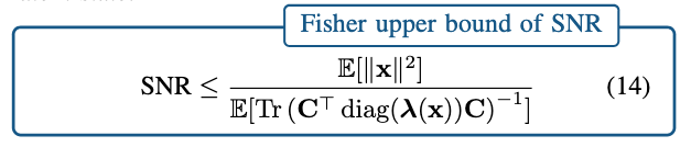
If the entries (“gain”) of observation matrix C is large and/or the firing rate of the neurons are large, the upper bound of the SNR is larger.

For a 3D simulated case, the sharpness of the tuning (measured by the norm of C matrix while holding the marginal firing rate constant) modulates the bound:

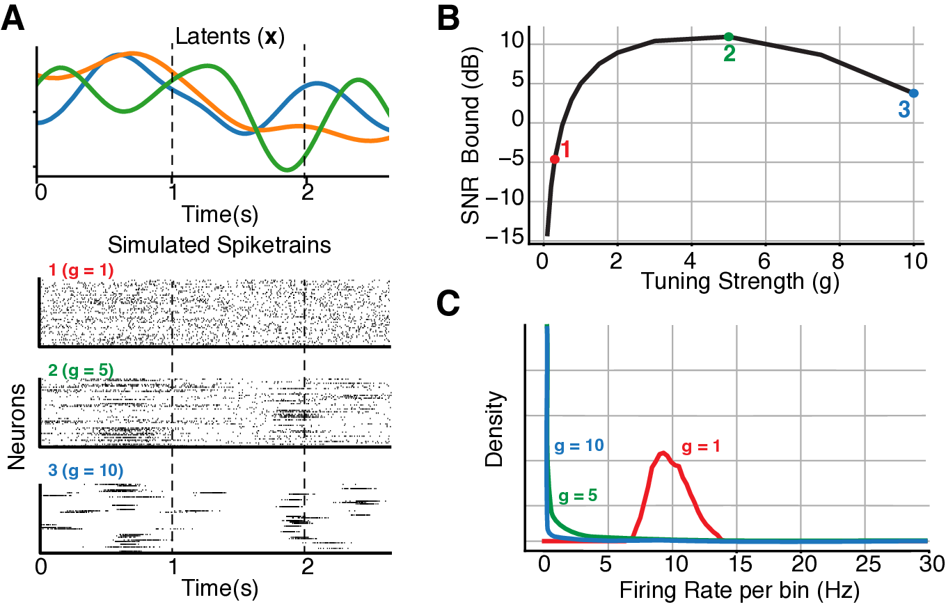
Note that intermediate amount of burstiness maximizes SNR.

We’ve applied these methods to publicly available dataset from the Neural Latent Benchmark, a neural population recording from dorso-medial frontal cortex (DMFC) while a monkey performs a time interval reproduction task (Sohn & Jazayeri 2022). To uncover the latent neural trajectories, we employed vLGP method (Zhao & Park 2017) to estimate the latents and C assuming smooth Gaussian Processes prior over the 3D latent trajectories x(t).

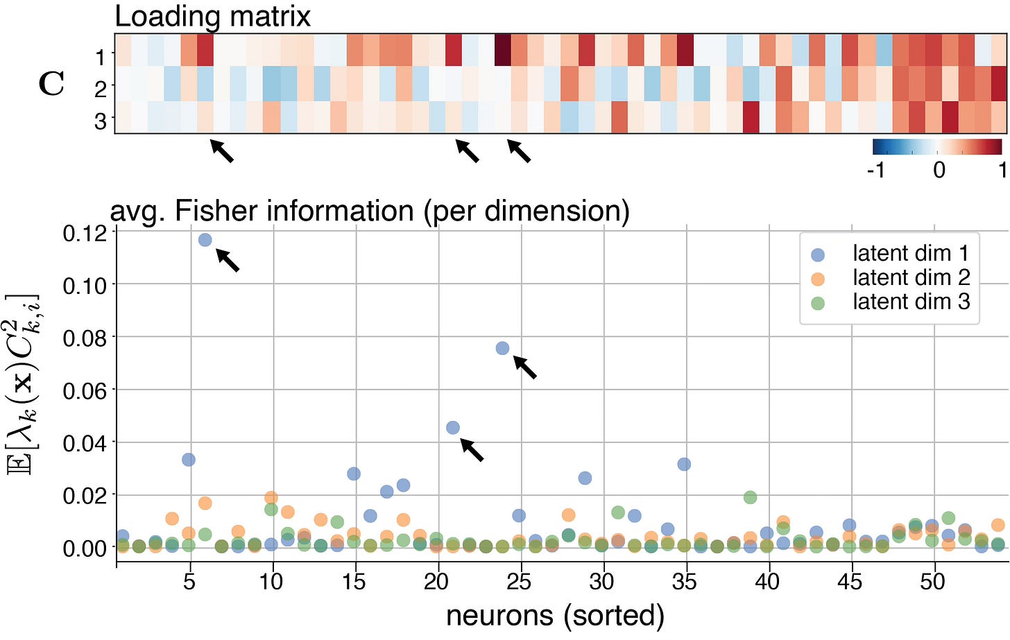
Instantaneous Fisher information shows directions in the latent space that are more informative and seem to correlate with the trajectories. (probably due to vLGP)

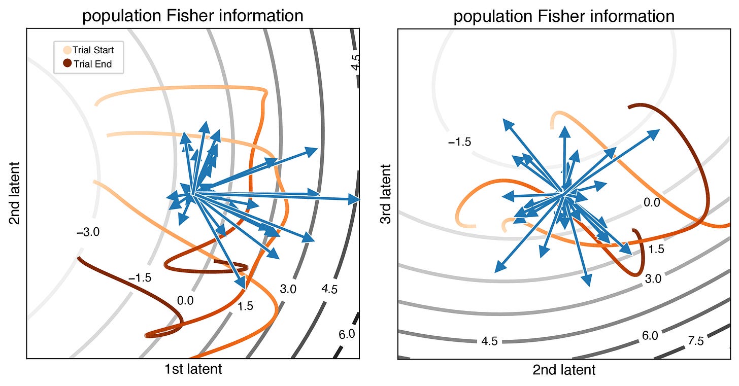
Interestingly, we found that the Fisher information is primarily dominated by a few neuron-latent pairs, indicating that “only a subset of the neurons strongly contributes to the overall information about the latent states” (black arrow).

From our model, the theoretical SNR bound was estimated to be around −7.60 dB on average for a 5 ms bin, reflecting a very low SNR. However, we can leverage the temporal correlation in the neural data to further enhance the SNR. When the dynamics change rapidly, with minimal temporal correlation, there is little to be gained in terms of improving SNR. On the other hand, in systems with slower dynamics, where neural activity evolves more gradually over time, we can leverage this smoothness to substantially increase the SNR, leading to more reliable reconstructions of the underlying neural trajectories.

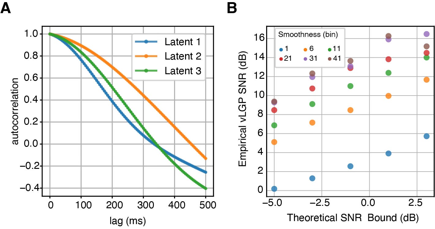
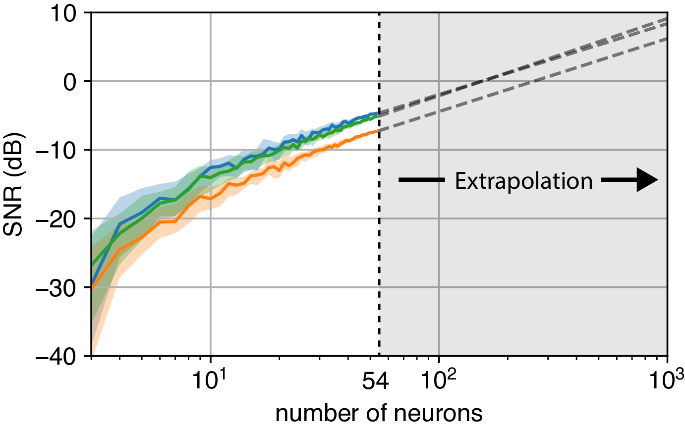
In addition to exploiting temporal structure, another effective method to improve the SNR is to record from a larger population of neurons. But this leads to an important experimental question: How many neurons do we need to record simultaneously to accurately reconstruct the latent neural states?

To address this, we subsample the recorded neurons and compute the corresponding SNR bound. Assuming that the loading matrix entries for unobserved neurons are independent and identical, we can then extrapolate the SNR to a larger population size, such as 1000 neurons. By fitting a power-law relationship, we provide a predictive model that allows experimenters to estimate the number of neurons required for reliable reconstruction of the underlying latent state. This approach offers a practical guide to determining the optimal scale for neural recordings in future experiments.

References

• Daley, D. J., & Vere-Jones, D. (1988). An Introduction to the Theory of Point Processes. Springer.

• Zhao, Y., & Park, I. M. (2017). Variational latent gaussian process for recovering single-trial dynamics from population spike trains. Neural computation

• Sohn, H; Jazayeri, M (2022) DMFC_RSG: macaque dorsomedial frontal cortex spiking activity during time interval reproduction task) [Data set]. DANDI archive.